Turning diode (and LED) datasheet IV plots into SPICE models

The SPICE models released by vendors are often really bad, producing results that do not anywhere near match the behaviour described in the datasheet. A recent example I ran into was for the CREE XLamp XP-E2 series LEDs, where the provided models underestimated the forward diode current by a factor of 6 compared to the datasheet and real-world measurements. Some vendors also don’t bother to release SPICE models at all, making it difficult to simulate the parts in LTspice.

Luckily, it is possible to turn the IV curve from a datasheet or a real-world measurement back into a SPICE model, and once you’ve figured out the necessary algebra (or someone else has figured it out for you) it is a fairly simple procedure. The result is a diode model that follows the IV curve correctly, which is primarily useful for LEDs but also comes in handy for applications like diode distortion pedals. Parameters like junction capacitance and transit time are not considered here, so you would need to derive those separately if you want to build models for switching applications (e.g. in a boost converter).

The Shockley diode equation is the core of the model. It is as follows:

$$I_D = I_S \left( e^{\frac{V_D}{n V_T}} -1 \right)$$

The forward current (I_D) is determined by the saturation current (I_S), the ideality factor (n), the voltage across the diode (V_D), and the thermal voltage (V_T). The thermal voltage parameter V_T is generally given as a constant 25.852mV at 300 Kelvin, which simplifies the maths a lot.

Given the saturation current and ideality factor parameters that describe a diode, and assuming constant temperature, the Shockley diode equation will tell you the forward current for any given forward voltage drop over the diode, or vice versa. In theory, this allows you to describe the IV curve using just two parameters. In practice, unfortunately, the Shockley diode equation as stated is only capable of describing ideal diodes, and real-world diodes are not ideal.

The critical parameter that is missing, at least for our purposes here, is parasitic series resistance (R_S). A real diode has some small internal resistance which causes the gradient of the IV curve to taper off at high forward bias. If we fit the ideal Shockley diode model (i.e. where R_S = 0Ω) to a series of points on the measured IV curve, we’ll find that the regression does not produce a close fit and the resulting model does not do a very good job of predicting the forward current for a given forward voltage. If we account for non-zero parasitic resistance, however, the regression typically produces a very close fit and the model’s predictions are fairly accurate.

Unfortunately, this parameter complicates things a bit. Ohm’s law tells us that the voltage drop over a resistor is proportional to the current flowing through it:

$$V = IR$$

But, looking at the Shockley diode equation above, the current flowing through the diode (and therefore the resistor too, since they’re in series) is proportional to the voltage drop over the diode. So in order to know the current flowing through the diode we need to know the voltage drop over it, but in order to know the voltage drop over the diode we first need to know the voltage drop over the resistor, which is determined by the current, leaving us in a catch-22.

It is possible to break this catch-22 by using (cue dramatic music) simultaneous equations. The non-ideal Shockley model can be stated as follows:

$$V_D - R_S \cdot I_D = n \cdot V_T \cdot \text{ln}\left( \frac{I_D}{I_S} - 1 \right)$$

This equation is derived by rearranging the ideal Shockley equation to be in terms of V_D instead of I_D, then subtracting the voltage drop of the resistor from the left side.

Simultaneous equations are not my favourite thing in the world, but thankfully there are tools we can use to avoid having to do the maths ourselves. This is particularly welcome here because practically solving a simultaneous equation where a term sits in a linear expression on one side and a logarithmic expression on the other involves something called the Lambert W function, which I have filed under the category of “things where I read the description on wikipedia and then felt like I understood the topic less than before I went in”. If you’re interested in playing with this further, you can attack this problem computationally using Halley’s method, and the GNU Scientific Library (GSL) has an implementation of the Lambert W functions, which has been ported to JS if you’d rather read that than the type of C that GNU folks tend to write.

Our saviour today is Desmos Graphing Calculator. Among the many incredible things it can do, it is capable of doing regressions over a table of points, even where the regression requires solving these difficult simultaneous equations.

Step one is to get the data points. If you’re working from a datasheet, you can take a screenshot of the IV curve and put it into WebPlotDigitizer. Set the X and Y axes up, making sure to specify the current scale in amps rather than milliamps. You can then add points manually along the line of interest, or use the automatic extraction feature by setting the foreground colour (use the picker in the popup to pick the exact colour from the graph) and using the Pen tool to highlight the line, then clicking Run. You can then use the Delete Point and Add Point tools to clean up any errant points - I tend to find the start and end of the line are where this happens the most. After you’ve got points drawn on the graph, click View Data on the left to get a table of points, and change the “Sort by” option to X.

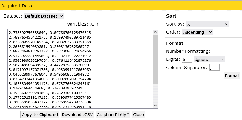
This gives us a series of points where the X axis is the forward voltage in volts and the Y axis is the forward current in amps.

These can be copy-pasted into a cell in the Desmos Graphing Calculator, which will automatically turn them into a table:

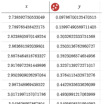
You should now add a subscript to the two variables, so x and y become x₁ and y₁ respectively. You can do this by typing an underscore after the variable name, e.g. x_1 to get x₁. This tells the calculator that these are specific data points relating to each other, rather than just abstract x and y values.

We can now run a regression over these points, using the simultaneous equation shown above, substituting V_D and I_D for x₁ and y₁ respectively:

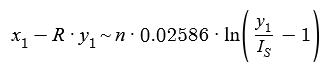
Note that a tilde has been inserted instead of an equals, which tells the calculator that we want to do a regression. The results of the regression are shown underneath:

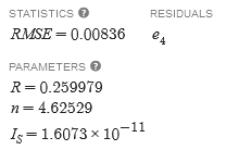
This tells us that the regression produced a fit with an RMS error of 0.00836, and that fit had a series reistance of 0.259979Ω, an ideality factor (n) of 4.62529, and a saturation current (I_S) of 1.6073x10^-11 amps. We can turn this into a SPICE model as follows:

.model OUR_FANCY_DIODE D
+ Is=1.6073e-11
+ N=4.62529
+ Rs=0.259979

The RMS error tells us how close the model fits our datapoints. 0.00836 is on the higher end of what I saw when building models from datasheets; many of the models had RMS errors closer to 0.001. I noticed that higher error numbers tended to be reported where the resolution of the source graph was low and therefore introduced a fair amount of quantisation error at low forward currents. Regardless, the resulting SPICE models match the datasheet IV curves very nicely, even when the RMSE is on the higher side.

If you want to take a look at some examples of models I built using this method, check out my CREE XLamp XP-E2 SPICE models and the Desmos Graphing Calculator sheet I used to build them.

I’m also working on a tool, to add to my existing repertoire of calculators, that automates generation of a SPICE model given datasheet parameters and the IV curve datapoints. Watch this space :)