The problem with driving LEDs with PWM
This blog post is a companion piece to my LED PWM Calculator web tool.
Your eyes are part of an evolutionary pathway that started more than half a billion years ago. Vision capable of accurately identifying objects and movements in the dark has proven to be a key asset when it comes to the chances of surviving the night in an environment filled with predators. This blog post is about LEDs, which are not generally considered to be predators. However, this millennia-long evolutionary process of biological adaptation is relevant if we want to study the relationship between the physical properties of light reaching our eyes and the perceptual results we observe as humans.
Luckily, if we want to understand these relationships at an applied level, we don’t need to borrow a few jars of eyeballs from the local teaching hospital and start putting retinas under microscopes. Other people have already done the hard work of studying the rods and cones, building models of the neurological activation behaviours under varying optical conditions, and turning those models into a set of standards and processes which we can use without getting our hands gooey. I am, of course, talking about the field of colourimetry.
Pulse width modulation (PWM) relies on our persistence of vision to act like a low-pass filter on very fast flickering images. If you flash an LED on and off at 1kHz, you won’t really perceive the flashing but will instead see the LED lit up dimly. By flashing the LED at a fixed frequency, but adjusting the percentage of each cycle that the LED spends turned on, the average amount of radiant power that the LED emits can be adjusted.
However, if you linearly sweep the duty cycle from 0-100%, you won’t see a smooth linear increase in brightness. This is because our eyes are far more sensitive to changes in brightness in the dark than in bright light; the evolutionary reasons for this are fairly obvious.
If you graph the PWM duty cycle versus the normalised perceptual brightness, you’ll get a curve that looks something like this:
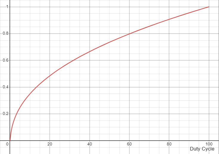
At just 5% duty cycle, the perceptual brightness of the LED already exceeds 20% of the maximum. At a 20% duty cycle, the perceptual brightness of the LED has almost reached 50% of the maximum.
To correct for this, we use gamma correction. Rather than mapping a brightness input of 0.0-1.0 linearly to a duty cycle of 0-100%, we take the inverse of the perceptual brightness curve and use it as a gamma correction function:
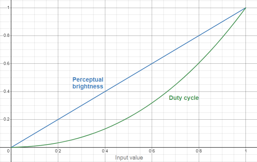
The simplest type of gamma correction function is of the following exponential form:
where γ is the gamma value; a common value for γ is 2.2.
If you take an input brightness level of 0.0 to 1.0 and run it through the gamma correction function, it’ll tell you the duty cycle that you should apply in order to achieve perceptual brightness linearity. For example, if I want the LED to be exactly half as bright as the maximum, I calculate 0.52.2 = 0.2176, which tells me that I should set the duty cycle to 21.76%.
A more general term for this kind of transformation is an electro-optical transfer function (EOTF).
For colour images (or RGB LEDs) we tend to talk about this in the context of a colour space. The sRGB colour space is one of the most commonly used - sRGB is almost certainly the colour space used by the device you are using to read this blog post. It’s the standard colour space for the web. For 8-bit per channel (8bpc) sRGB there are 256 possible values each for red, green, and blue. These values are gamma-compressed with the sRGB EOTF, such that they are perceptually linear - if you double the value for one of the RGB channels, e.g. going from [0,64,0] to [0,128,0], the perceptual brightness of that channel doubles. Your graphics processor or display then translates those sRGB values back into linear RGB values using the EOTF, in hardware, in order to figure out how bright each of the physical primary elements (red, green, and blue) of the pixels in your display should be.
The sRGB EOTF isn’t a simple exponential gamma function. Instead, the function starts with a linear gradient of 1/12.92 in the first 4.045% of the perceptual brightness space, then switches to an exponential gamma of γ=2.4 for the remainder of the transfer function.
As it turns out, this is extremely close to just using a simple gamma of γ=2.2. So close, in fact, that a lot of people don’t bother to implement the correct sRGB EOTF, and instead use the simpler approximation. The short linear section at the start of the sRGB EOTF is a better representation of how we see very small brightness changes when the LED is almost completely switched off, but if you don’t care about displaying very dim images (or patterns) then it might not matter at all.
The problem, though, is quantisation. When we quantise the perceptual colour space into 8 bits per channel, like we do with sRGB colours on the web (and most other computer stuff), everything is mostly fine. Each quantised step represents an equal change in perceptual brightness - one 256th of the range, or 0.391%. However, if you quantise in the linear space, each step no longer represents an equal change in perceptual brightness. If you’re dimming an LED with an 8-bit PWM controller, the first step represents a 4.97% increase in brightness, the second step represents a 3.5% increase in brightness, and the third step represents a 2.57% increase in brightness.
This graph shows the perceptual brightness values that can be represented as a result of using 8-bit quantisation in linear brightness space:
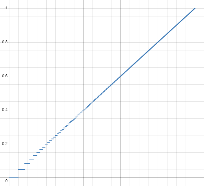
Notice how much stepping there is in the lower range? Rather than having 128 steps in the bottom half of the perceptual brightness range, and 128 steps in the upper half of the perceptual brightness range, the linear quantisation causes a significant skew: 55 steps in the lower and 201 steps in the upper. The bottom 20% of the perceptual brightness range only has 8 steps!
The minimum non-black perceptual brightness that such a system can display is 4.97%, which produces a contrast ratio of only 20:1 over the lit range. If we were quantising in sRGB space rather than linear space, the minimum non-black perceptual brightness would be 0.39% and the contrast ratio would be 256:1 over the lit range.
A quick note on terminology: for subtractive display technologies, like LCD, the contrast ratio specification refers to the ratio between the intensity of backlight bleed at the black level and the maximum intensity of the white level. This measurement doesn’t make any sense for emissive technologies like LEDs, which have “infinite” contrast ratios because the black level emits no visible light at all - any amount of white intensity divided by zero is infinity. You’ll often hear people refer to OLED panels as having infinite contrast ratio for this exact reason. Since LEDs driven by quantised linear PWM suffer from stepping at the dimmest end, we can repurpose the contrast ratio metric by measuring the ratio between the lowest non-black perceptual brightness and the highest perceptual brightness.
As a result of this nonlinearity, if you try to display a smooth gradient on an LED driven with 8-bit quantised linear PWM you’ll find that it flickers and steps quite a lot. This doesn’t just affect the dimmest colours, but any colour where one channel is near zero. This is essentially identical to the problem of colour banding on TVs and monitors. This problem is one of the reasons why it’s so difficult to get off-the-shelf RGB LEDs like WS2812B to look good.
So, how do we fix this? Well, we could genetically engineer ourselves to have linear optical sensors, but getting a PhD in genetics and fighting off the anti-transhumanism luddites seems like a hassle. Luckily for us, there’s a simpler way: more bit depth!
At 10-bit linear depth we end up with 219 steps in the lower half of the perceptual brightness range, which seems like it would outperform 8-bit quantisation in the sRGB colour space, which “only” has 128 steps. However, despite having 219 steps in that lower half, they aren’t linearly distributed. The bottom 20% of the perceptual space still only has 20 steps, and the minimum perceptual brightness is 1.26%, leading to a contrast ratio of 79:1 - far worse than the 0.39% and 256:1 achieved by perceptually quantised sRGB.
12-bit linear quantisation is the point where we meet (and slightly outperform) 8-bit perceptual quantisation with sRGB across the full range. The minimum perceptual brightness is 0.32% and the contrast ratio is 317:1. So, if you want your linear PWM dimmers to look as smooth as a regular monitor, go with 12-bit quantisation.
You can tinker around with these numbers using my LED PWM calculator, which I wrote specifically to figure out these numbers and, as we’ll discuss next, the tradeoffs involved.
There is a downside to greater bit depth: every time you add a bit, the minimum pulse duration is halved. This doesn’t sound that bad until you think about the multiplicative effect of frequency and bit depth. The pulse duration calculation is:
For 8-bit PWM at 1kHz, the minimum pulse time is 3.91μs. For 12-bit PWM at 1kHz, the minimum pulse time is 244ns. That’s quite a short time period - the equivalent pulse frequency jumped from 256kHz to 4.1MHz. At 16-bit you’ve got a pulse period of just 15.26ns, corresponding to 65.54MHz - a heck of a lot more than the 1kHz PWM rate.
A major challenge with higher bit depths is the rise and fall times (tr/tf) of the driver, especially on LEDs that pull more than a few milliamps. Consider the 12-bit 1kHz case mentioned above - a minimum pulse time of 244ns means that, in order to meet a timing accuracy of 20%, the rise and fall times of the driver cannot exceed 24ns. For a 3V / 50mA LED that’s a voltage slew rate of 245V/μs and a current slew rate of 4.1A/μs. This quickly enters the realm of having to carefully consider MOSFET gate charge, gate driver performance, and power delivery network impedance.
To increase the minimum pulse time and reduce the required tr/tf of the driver, we could reduce the PWM frequency. This works, but it doesn’t scale very well - each additional quantisation bit makes the required tr/tf twice as tight, but the effect of PWM frequency is linear, so if you try to keep halving the frequency you’ll end up with a very flickery result across all brightness levels, which looks worse than less quantisation.
An alternative approach is to use temporal dithering. Temporal dithering works by altering the least significant bit (LSB) of the PWM value on each cycle to achieve an intermediate value on average. With 1-bit temporal dithering it is possible to achieve an average intensity half way between two integer states by swapping between the two. For example, to reach a value of 21.5 you would flip between 21 and 22 on each cycle.
Temporal dithering can be extended to longer patterns in order to attain more intermediate values. 2-bit dithering uses a pattern length of 4 (i.e. 22) to achieve intermediate values of 0.25, 0.5, and 0.75:
| Pattern | Number of set bits | Intermediate value |
| 0001 | 1 | 0.25 |
| 0101 | 2 | 0.5 |
| 1110 | 3 | 0.75 |
For example, to achieve an average value of 8.25, the pattern of duty cycles would be [8, 8, 8, 9].
3-bit dithering uses a pattern length of 8 (i.e. 23) to extend this further:
| Pattern | Number of set bits | Intermediate value |
| 00000001 | 1 | 0.125 |
| 00010001 | 2 | 0.25 |
| 01001001 | 3 | 0.375 |
| 01010101 | 4 | 0.5 |
| 10110110 | 5 | 0.625 |
| 11101110 | 6 | 0.75 |
| 11111110 | 7 | 0.875 |
For example, to achieve an average value of 8.375, the pattern of duty cycles would be [8, 9, 8, 8, 9, 8, 8, 9].
Temporal dithering effectively increases the bit depth of the driver without altering the timing requirements of the linear PWM driver itself. Some processor overhead is required in order to change the duty cycle on each PWM cycle, but at 2kHz this only involves running a few instructions every 500μs, which should be trivially achievable with even the cheapest of 8-bit MCUs.
There is, however, a limit to how far we can go with temporal dithering. If the duration of the dithering pattern exceeds the frame period (e.g. 16.67ms for 60fps) then the averaged duty cycle across one frame period will be incorrect. In addition, the temporal dithering will cause brightness ripple at a frequency proportional to the length of the pattern:
where fR is the ripple frequency and d is the number of temporal dithering bits.
At 1kHz PWM, 4-bit temporal dithering will cause ripple in the range of 62.5Hz to 500Hz. The magnitude of temporal dithering ripple depends on the amount of linear quantisation and the exact duty cycle value being displayed. At low duty cycles, the magnitude of dithering ripple will be closer to the minimum perceptual brightness step before temporal dithering is applied. Stroboscopic effects will generally become quite noticeable below 400Hz if the change in perceptual brightness between cycles is non-negligible. The stroboscopic effects are particularly impactful during saccades and can be very nauseating if your LEDs are bright. Remember the early days of LED light bulbs? Yeah, that sucked.
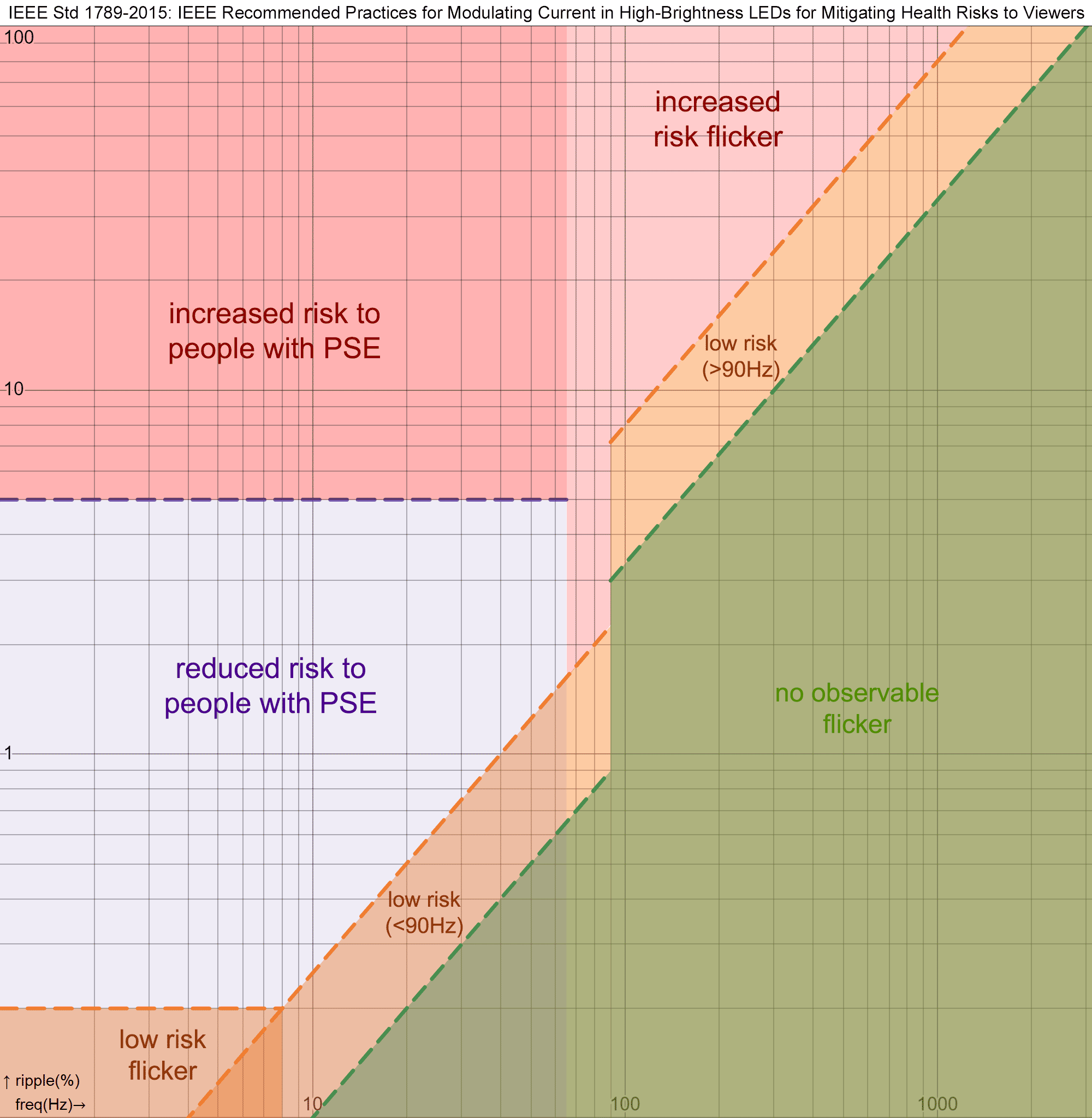
Update (2023-07-20): I have now added risk category calculations for flicker to the calculator, based on IEEE 1789 “IEEE Recommended Practices for Modulating Current in High-Brightness LEDs for Mitigating Health Risks to Viewers”. The standard defines a set of risk regions based on the relationship between the modulation depth of flicker (Michelson contrast, in percent) and the frequency of the flicker. Separate categorisation is performed for human observers in general, and for viewers with photosensitive epilepsy (PSE).
All these behaviours result in a trade-off between linear bit depth, temporal dithering bit depth, PWM frequency, and driver timing. Picking the correct parameters for your application is a matter of balancing colour performance against the technical complexity and cost of the driver.
If you need perceptual linearity beyond what simple PWM can reasonably offer, there are a couple of alternative options for LED drivers.
The first alternative is a linear constant-current driver. Rather than using a PWM driver, a DAC can be used to output a continuous analog voltage which sets the amount of current provided by the driver. The DAC’s own quantisation in linear space will still apply, but since there’s no PWM involved and the DAC only needs to update at the target frame rate, supplying just a few nanoamps of current in the control signal, it’s far less challenging to get 12-bit depth or better. The trade-off is efficiency. A linear constant-current driver achieves the voltage drop necessary to meet the target current by burning power as heat. You also need a separate linear regulator per independently controllable LED, which may be more expensive than using PWM.
Another alternative is a switch-mode constant-current driver. This can be controlled in a similar way, using a DAC to set the current, but has the benefit of being far more efficient. Switch-mode controllers essentially use PWM to produce a constant average output current, using the output inductor and capacitor as a kind of LC low pass filter. However, these controllers are far more advanced than a simple PWM LED driver, and achieve switching frequencies in the hundreds of kHz or even a few MHz. They come with downsides, though: cost, complexity, and board space. If you need to control a dozen LEDs, you’ll need a dozen separate switch-mode constant current drivers. If you’re designing a commercial product, this also makes it very challenging to comply with conducted emissions standards.
You can also look for specialised LED driver chips or programmable LEDs that support gamma correction bits in hardware. These typically split the bit depth into two parts: upper bits that index a piecewise linear function approximating a gamma curve, and lower bits that interpolate across each linear piece. I put together a quick demo of the PWL gamma approximation on Desmos, so you can tweak the gamma bit depth and see how the linear segments fit the gamma curve. The gamma portion of the bit depth specifies which linear piece is active, and the linear portion of the bit depth interpolates across that linear piece. With enough gamma correction bits the approximation can be very good. One example of this in practice is the WS2816B addressable LED, which has 16-bit depth split into 4-bit gamma and 12-bit linear control. This lets us treat the whole 16-bit control value as being in perceptual space. However, the gamma value / EOTF approximated by the PWL is not specified in the datasheet, so if you need colourimetric accuracy (e.g. matching other light sources, or attaining a D65 whitepoint) they might not be suitable. Other drivers offering similar PWL-based gamma correction do specify their EOTF, and may even let you customise the gamma value.
Finally, I’d like to talk about analogue gamma correction. There’s a circuit that’s been floating around the internet since the late 90s, which combines the I/V transfer curve of several diodes to produce a gamma-like response curve. It comes up quite frequently when the topic of LED gamma correction is discussed. I’ve simulated this gamma correction circuit, and you can see the results below:
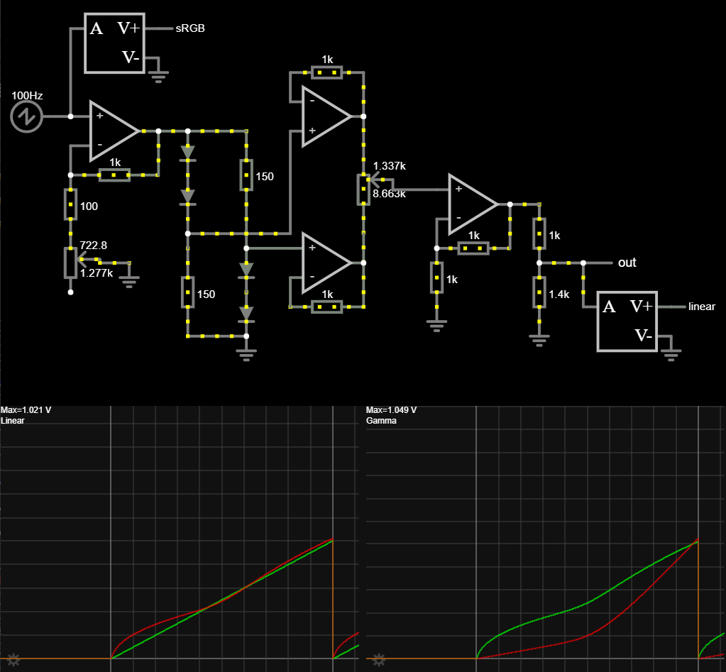
The green line on the left graph is the linear input. The red line on the left graph is the resulting perceptual brightness. The green line on the right graph is the gamma compressed value. The red line on the right is what the gamma compressed value should really be. My apologies to colour blind folks; Falstad only has red and green traces as options. Deuteranopia notwithstanding, it should be clear from the divergence of the lines that this isn’t a very accurate way to implement an EOTF. You can tweak the two potentiometers to try to get it closer, but it’s impossible to get perfectly right. Environmental temperature variations will cause significant skew, and each correction circuit requires manual calibration to account for part tolerances and variations. This circuit was originally designed for gamma correction in analogue TV broadcast receivers and really isn’t suitable for LEDs.
If you’d like to know more about specific fields in the LED PWM calculator, you can view descriptive information by hovering over the label (or the little [i] icon on mobile browsers). If you need more clarification, feel free to message me on Mastodon (@gsuberland@chaos.social).